
EvoMath 3: Genetic Drift and Coalescence, Briefly
Genetic Drift
EvoMath is back from a long hiatus. In this edition I will briefly touch on genetic drift and coalescence theory. Genetic drift is the evolutionary force whereby allele frequencies fluctuate due to chance because the alleles in a generation are a random sample of the alleles in previous generation. To help understand what I am talking about, consider a heterozygous father, with genotype Aa. Under Mendelian heredity, he will pass on the A allele 50% of the time and the a allele the other 50% of the time. If he has only one child, then he clearly cannot pass on both of his alleles, and thus one of those alleles–say a–will be lost from his lineage. The remaining allele, A, will then have “drifted” to 100% or “fixation.” If he has more children, then he may pass on both of his alleles, but it is not likely to be exactly at a 50:50 ratio.
Genetic drift occurs whenever a population has a finite size, and since all populations are finite, it occurs in all populations. However, in large populations it can be very weak and thus negligible compared to other evolutionary forces.
To model genetic drift, first assume Hardy-Weinberg conditions except that the population has a constant, finite size of \(N\). Let \(N_g\) be the number of genes competing at a locus. (\(N_g=2N\) for diploids. \(N_g=N\) for haploids.) In each generation the population is in a certain state, which corresponds to the frequency of the A allele. Assume that the genotype of each offspring is independent of all other offspring, i.e. the chance that an individual will be the parent of an offspring does not depend on how many offspring it already has. Then the process of reproduction is simply “sample with replacement” and thus has a binomial distribution. More specifically, if the current frequency of allele A is \(p\), then the probability mass function of the allele frequency in the next generation, \(p^\prime\), is
\[\Pr\left\{p^\prime = n / N_g \mid p \right\} = \frac{N_g!}{n! \left( N_g-n \right) !}p^n {\left( 1-p \right)}^{N_g-n} \mbox{ if } n = 0,1,\ldots,N_g.\]From this equation it is easy to see that the boundaries, \(p=1\) and \(p=0\), are two special situations: \(\Pr\left\{p^\prime = 1 \mid p = 1 \right\} = 1\) and \(\Pr\left\{p^\prime = 0 \mid p = 0 \right\} = 1\). This means that if an allele frequency drifts to a boundary, it stays there. Biologically, the boundaries represent the states where one allele has gone extinct and the other allele has gone to fixation. Since there is no mutation in the model, once an allele is lost, it is lost for good. Statisticians call states where a process is able to enter but not leave “absorbing states.” The classic explanation of this process is “the dipsomaniac’s stumble.”
Imagine a drunken man walking along a bridge with no railing. Because he is inebriated, he randomly takes steps to the right and the left. Eventually he will come to the right or left edge of the bridge and fall off being absorbed by the river.
My house has its own version of a random process with absorbing states: “the cats’ amusement.” We have two cats, Isabelle and Precious, and they have toy mice, which they playfully knock around the house. Eventually they lose all their toy mice, and either my wife or I have to dig them out from under one of their absorbing states: the refrigerator or the bookcase.
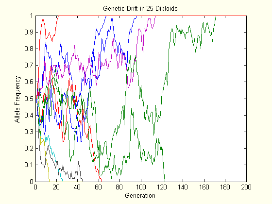
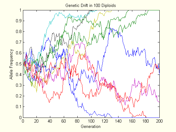
The above charts each show the evolution of ten populations via genetic drift. Each population starts at \(p=0.5\), and their trajectory is followed for two hundred generations. As one can see, the allele frequency randomly fluctuates until it hits either boundary, and this happens slower in the larger population.
Coalescence
Instead of looking at just two alleles, we can look at each gene in a population separately, as if each one was its own, unique allele. Below are three simulations of a population of four individuals where genetic drift is the only evolutionary force. Bold represents the lineage that goes to fixation.
| Generation: | 1 | 2 | 3 | 4 | 5 | 6 | 7 | 8 | 9 | 10 | 11 | 12 | 13 | 14 | 15 | 16 | 17 | 18 | 19 | 20 |
|---|---|---|---|---|---|---|---|---|---|---|---|---|---|---|---|---|---|---|---|---|
| Genes: | 1 | 1 | 1 | 1 | 1 | 1 | 1 | 1 | 1 | 1 | 1 | 1 | 1 | 1 | 1 | 1 | 1 | 1 | 1 | 1 |
| 2 | 1 | 1 | 1 | 2 | 1 | 1 | 1 | 1 | 1 | 1 | 1 | 1 | 1 | 1 | 1 | 1 | 1 | 1 | 1 | |
| 3 | 2 | 2 | 2 | 6 | 2 | 1 | 1 | 1 | 1 | 1 | 1 | 1 | 1 | 1 | 1 | 1 | 1 | 1 | 1 | |
| 4 | 6 | 6 | 6 | 6 | 7 | 2 | 2 | 2 | 1 | 1 | 1 | 1 | 1 | 1 | 1 | 1 | 1 | 1 | 1 | |
| 5 | 7 | 7 | 7 | 7 | 7 | 7 | 2 | 2 | 7 | 1 | 1 | 7 | 7 | 1 | 1 | 1 | 1 | 1 | 1 | |
| 6 | 7 | 7 | 8 | 7 | 7 | 7 | 7 | 7 | 7 | 7 | 1 | 7 | 7 | 1 | 1 | 1 | 1 | 1 | 1 | |
| 7 | 8 | 8 | 8 | 8 | 8 | 8 | 8 | 7 | 7 | 7 | 7 | 7 | 7 | 7 | 7 | 1 | 1 | 1 | 1 | |
| 8 | 8 | 8 | 8 | 8 | 8 | 8 | 8 | 8 | 8 | 7 | 7 | 7 | 7 | 7 | 7 | 1 | 1 | 1 | 1 |
| Generation: | 1 | 2 | 3 | 4 | 5 | 6 | 7 | 8 | 9 | 10 | 11 | 12 | 13 | 14 | 15 | 16 | 17 | 18 | 19 | 20 |
|---|---|---|---|---|---|---|---|---|---|---|---|---|---|---|---|---|---|---|---|---|
| Genes: | 1 | 2 | 2 | 2 | 5 | 5 | 5 | 5 | 5 | 5 | 5 | 5 | 5 | 5 | 5 | 5 | 5 | 5 | 5 | 5 |
| 2 | 2 | 2 | 2 | 5 | 5 | 5 | 5 | 5 | 5 | 5 | 5 | 5 | 5 | 5 | 5 | 5 | 5 | 5 | 5 | |
| 3 | 3 | 5 | 5 | 5 | 5 | 5 | 5 | 5 | 5 | 5 | 5 | 5 | 5 | 5 | 5 | 5 | 5 | 5 | 5 | |
| 4 | 4 | 5 | 5 | 8 | 5 | 5 | 5 | 5 | 5 | 5 | 5 | 5 | 5 | 5 | 5 | 5 | 5 | 5 | 5 | |
| 5 | 4 | 5 | 5 | 8 | 5 | 5 | 8 | 5 | 5 | 5 | 5 | 5 | 5 | 5 | 5 | 5 | 5 | 5 | 5 | |
| 6 | 5 | 8 | 8 | 8 | 8 | 8 | 8 | 5 | 5 | 5 | 8 | 8 | 5 | 8 | 5 | 5 | 5 | 5 | 5 | |
| 7 | 5 | 8 | 8 | 8 | 8 | 8 | 8 | 8 | 8 | 5 | 8 | 8 | 8 | 8 | 8 | 5 | 5 | 5 | 5 | |
| 8 | 8 | 8 | 8 | 8 | 8 | 8 | 8 | 8 | 8 | 8 | 8 | 8 | 8 | 8 | 8 | 5 | 5 | 5 | 5 |
| Generation: | 1 | 2 | 3 | 4 | 5 | 6 | 7 | 8 | 9 | 10 | 11 | 12 | 13 | 14 | 15 | 16 | 17 | 18 | 19 | 20 |
|---|---|---|---|---|---|---|---|---|---|---|---|---|---|---|---|---|---|---|---|---|
| Genes: | 1 | 1 | 1 | 4 | 4 | 4 | 4 | 4 | 4 | 4 | 4 | 4 | 4 | 4 | 4 | 4 | 4 | 4 | 4 | 4 |
| 2 | 4 | 4 | 4 | 4 | 4 | 4 | 4 | 4 | 4 | 4 | 4 | 4 | 4 | 4 | 4 | 4 | 4 | 4 | 4 | |
| 3 | 4 | 4 | 4 | 4 | 4 | 4 | 4 | 4 | 4 | 4 | 4 | 4 | 4 | 4 | 4 | 4 | 4 | 4 | 4 | |
| 4 | 5 | 4 | 4 | 4 | 4 | 4 | 4 | 4 | 4 | 4 | 4 | 4 | 4 | 4 | 4 | 4 | 4 | 4 | 4 | |
| 5 | 6 | 4 | 4 | 4 | 4 | 4 | 4 | 4 | 4 | 4 | 4 | 4 | 4 | 4 | 4 | 4 | 4 | 4 | 4 | |
| 6 | 7 | 4 | 4 | 5 | 4 | 4 | 4 | 4 | 4 | 4 | 4 | 4 | 4 | 4 | 4 | 4 | 4 | 4 | 4 | |
| 7 | 7 | 5 | 5 | 5 | 4 | 4 | 4 | 4 | 4 | 4 | 4 | 4 | 4 | 4 | 4 | 4 | 4 | 4 | 4 | |
| 8 | 7 | 7 | 7 | 7 | 7 | 4 | 4 | 4 | 4 | 4 | 4 | 4 | 4 | 4 | 4 | 4 | 4 | 4 | 4 |
As you can see, all “alleles” but one are eventually lost from the population. However, each “allele” represents a separate gene from generation 1, thus the descendents of one gene have replaced all other lineages at the locus. This process is known as “coalescence.” As you can see from the separate simulations, coalescence is not always the same. Although the simulations are forwards in time, we can look at it backwards in time. For every gene currently in the population, there exists a common ancestor some time in the past.
Now, if we think of each simulation as a separate genetic locus in the same population, then it follows that the coalescent lineage of different loci can be different. What this means is that there are multiple “most recent common ancestors” for any population, each one associated with a region of the genome. A common misconception of the coalescent is that it signifies that there was only one individual alive in the population at that time. This is especially popular in writings about “mitochondrial Eve.” As you can see from the simulations, this is not true. The coalescent simply represents the lineage out of many that “won.”
Since coalescence is inevitable, the probability that any one gene is the one that eventually “wins” is clearly \(1 / N_g\), and the probability that any one gene eventually “loses” is \(\left(N_g-1 \right) / N_g\). Similarly the probability that any allele eventually goes to fixation is \(p\), and the probability that any allele eventually goes to extinction is \(1-p\), where \(p\) is the current frequency of that allele in the population.
It can be shown that the average time to the most recent common ancestor of random pairs of genes in a population is \(N_g\) generations. It is clear from this that coalescence occurs faster in smaller populations, as we saw earlier. Likewise, the average time to the most recent common ancestor of all genes is \(2N_g\) generations. Together, these two equations tell us that most of the time is spent waiting for the last two lineages to coalesce.
The rate of coalescence among \(k\) genes in a population of \(N_g\) genes is approximately \(k \left( k-1 \right) / 2N_g\), as long as \(N_g \gg 2 k \left(k-1\right)\). (Actual derivation is for another evomath.) From this it follows that the number of generations until the next coalescent event is approximately exponentially distributed with mean \(2N_g / k \left( k-1 \right)\). Furthermore, the expected time in generations to the most recent common ancestor of all \(k\) individuals is
\[\begin{split} E \left( TMRCA \right) &= \frac{2N_g}{k \left( k-1 \right)} + \frac{2N_g}{\left( k-1 \right) \left( k-2 \right)} + \ldots + \frac{2N_g}{2} \\ &= 2N_g \left( \frac{1}{k-1} - \frac{1}{k} + \frac{1}{k-2} - \frac{1}{k-1} + \ldots + \frac{1}{1} - \frac{1}{2} \right) \\ &= 2N_g \left(1 - \frac{1}{k} \right) \end{split}.\]A rather simple algorithm (due to J.F.C. Kingman) can be used to simulate the coalescence process.
- Start with \(g=0\) as the “depth” of the tree.
- Draw a random number, \(t\), from an exponential distribution with mean \(2N_g / k \left( k-1 \right)\).
- Set \(g=g+t\).
- Decrease \(k\) by 1.
- If \(k=1\), stop. Otherwise, go to step 2.
When this ends, \(g\) will be your simulated time to most recent common ancestor. Modifications of this algorithm can be used to create graphs of coalescent lineages.
The basal split (caused by the root) of a random tree with \(k\) tips can have anywhere from \(1\) to \(k-1\) tips on the left-hand side. It can be shown that these values are equally probable. Using this we can determine how the addition of another tip to the tree will affect the location of the root. If we have fifty lineages and add a new one, will this lineage connect to the tree below the current root? The probability that the basal split has fifty lineages on one side and one lineage on the other is simply \(2/50\). The probability that the new lineage is the lone one is \(1/51\). Together, these indicate that the probability that adding a fifty-first tip actually increases the depth of the root is \(2/\left(50 \times 51\right)=0.000784\). Not all that significant of a difference, is it?
Previous Installments
- EvoMath 2: Testing for Hardy-Weinberg Equilibrium
- EvoMath 1: The Hardy-Weinberg Principle
- Genetic Drift: Futuyma D (1998) Evolutionary Biology ch11. Sinauer Associates, Inc.
- Coalescence: Felsenstein J (2004) Inferring Phylogenies ch26. Sinauer Associates, Inc.