
Icons of ID: Markov processes and nested hierarchies
I will explore how evolutionary processes by virtue of being Markov processes, are expected to generate nested hierarchies. In fact, I argue that evolutionary processes are the only known processes which can generate such nested hierarchies. On the ARN discussion boards we have seen much confusion as to the nature of evolutionary processes, nested hierarchies and common descent. It is trivial to show that a process of inheritance with variation (and selection) will generate a nested tree. The problem however is recovering the correct tree using only present day genetic data. That evolution is a Markov process is self evident. First inheritance depends solely on the parents and not on all the preceding ancestors, secondly transitions in DNA can be described by probabilities. This means that evolution is memory-less.
From Theobalt’s 29+ Evidences for Macroevolution FAQ
As seen from the phylogeny in Figure 1, the predicted pattern of organisms at any given point in time can be described as “groups within groups”, otherwise known as a nested hierarchy. The only known processes that specifically generate unique, nested, hierarchical patterns are branching evolutionary processes. Common descent is a genetic process in which the state of the present generation/individual is dependent only upon genetic changes that have occurred since the most recent ancestral population/individual. Therefore, gradual evolution from common ancestors must conform to the mathematics of Markov processes and Markov chains. Using Markovian mathematics, it can be rigorously proven that branching Markovian replicating systems produce nested hierarchies (Givnish and Sytsma 1997; Harris 1989; Norris 1997). For these reasons, biologists routinely use branching Markov chains to effectively model evolutionary processes, including complex genetic processes, the temporal distributions of surnames in populations (Galton and Watson 1874), and the behavior of pathogens in epidemics.
Lets first look at a phylogenetic tree
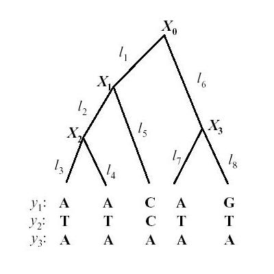
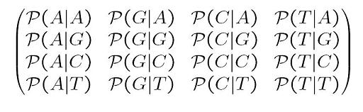
| x0 is the ancestral state. We can define a substitution rate matrix M which models the transition probabilities. For DNA for each nucleotide, there are four possible states A, C, T, G but the model can also be applied to amino acids in which case there are 20 states. We can now define transition probabilities _p(A | A), p(A | C), p(A | T), p(A | G)_ etc which model the probability of a transition from A to A, C, T and G respectively. We can thus define a matrix M as follows |
This model is the most generalized model and we can apply if necessary various simplifications such as a uniform distribution at the root, stationary distribution, or even special matrix forms. Historically there are some interesting matrix forms to consider: Jukes-Cantor, Kimura and Tamura
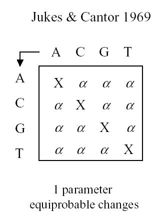
Jukes and Cantor have a single parameter assuming that the probability of change between any base-pair and any other base-pair is equiprobable. All sites are assumed to change independently
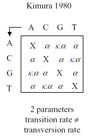
Kimura has two parameters, with different rates for transversion and transition.
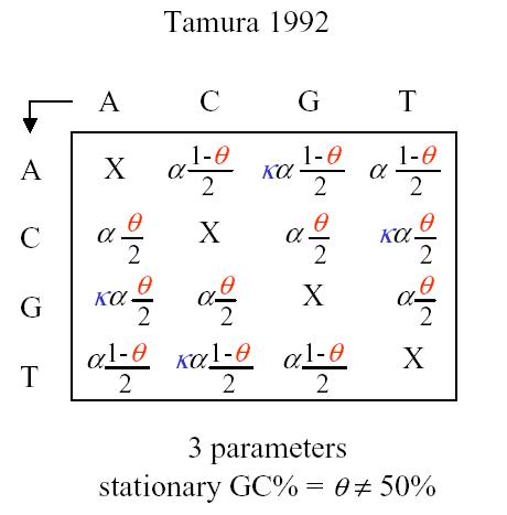
Tamura has a 3 parameter model
The most general model has 12 differente parameters, one for each transition, all the way down to the Jukes-Cantor model with only one parameter.
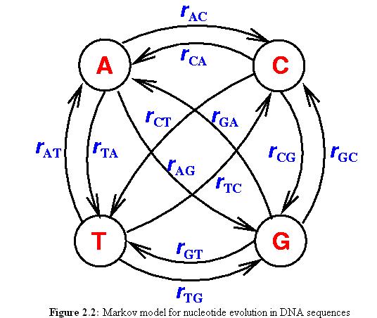
12 parameter model
Additionally since the rates are not even constant among sites, one can model this variation using for instance a gamma distribution. And finally one can have autocorrelations between neighboring sites having a similar rate of change. Using an appropriate model, one can incorporate all these variations.
One can actually test for rate changes see for instance Testing for Differences in Rates-Across-Sites Distributions in Phylogenetic Subtrees. Needless to say, phylogenetic models can capture variable rates quite easily.
Of course we can add further extensions to the model. The model so far looks at nucleotide changes but it can also incorporate inversions, transpositions etc.
Markov chains and processes
Now that we have discussed the Markov Matrix M, I will discuss Markov models in more detail. Basically a Markov model defines a state and the future state is determine solely by the present state. Let me repeat this. A Markov model states that it does not really matter how a particular state was reached, the future state will only depend on the present state, not on any preceding states. In other words, a Markov process is characterized by a state vector \(X\) and a matrix with transition probabilities \(p_{ij}\). Here \(p_{ij}\) is the probability that the state at the next time step will become \(j\) when it was \(i\). The transition probability matrix has some special properties namely that the rows of the probabilities sums to be 1. A Markov chain is a discrete time model while a Markov processes is a continuous time model.
\[{\bf X}(T+dT) = {\bf X}(T)({\bf I}+{\bf M}dT)\]where \({\bf I}\) is the identify matrix and \({\bf M}\) the Markov matrix described above. In this case the state at time \(T + dt\) is the product of the state at time \(T\) and a transition matrix. The state space vector \(X\) for these processes typically consists of 4 (nucleotides A, C, T and G) or 20 (aminoacids) . This Markov process is a ‘stochastic process’ as it gives you the distribution of nucleotides or aminoacids as funciton of time. Although I stated that Markov processes only depend on the current state, one can extend the paradigm to include one or more previous states by extending the state vector. Instead of for instance 4 parameters to describe the nucleotides at time \(T\) one could have 8 parameters, 4 to represent present time and 4 to represent the state at one time step earlier.
So in other words, a Markov process describes how a probability distribution of stochastic variables evolves as function of time. One simply multiplies the state space vector (which contains the probabilities) with the transition matrix to obtain the state space vector at the next time step.
For evolutionary processes the transition matrix models the likelyhood of nucleotide substitutions. As shown the model can be as simple as a single parameter model all the way up to a 12 parameter model. And that is for procesess where the probabilities are neither time nor location dependent.
Markov processes can have three important properties: homogeneity, stationarity and reversibility. Homogeneity means that the Markov matrix is independent of time, stationarity means that the nucleotide frequencies have remained at an equilibrium and reversibility means that the process can move in reverse with similar results.
Conclusions
Unless dealing with saturation, phylogenetic reconstruction models can reliably recover ancestral states and other relevant evolutionary parameters while taking into consideration a variety of assumptions and restrictions. That evolutionary processes form a Markov process and thus predict nested hierarchies means that the validation of said prediction by phylogenetic reconstruction methods is a powerful validation of evolution.
Links
Petri nets AN INTRODUCTION TO MARKOV CHAINS FOR INTERESTED HIGH SCHOOL STUDENTS by HALVERSCHEID
PyEvolve is an object-oriented toolkit designed to perform existing, and for the development of new, methods of molecular evolutionary analysis. The functional capabilities of PyEvolve are centered on its ability to perform phylogeny-based maximum-likelihood calculations. PyEvolve implements a range of existing and several novel Markov models of substitution (nucleotide, dinucleotide, codon, protein, and models for measuring interactions between sites) that can be used for these calculations. See also PyEvolve: a toolkit for statistical modelling of molecular evolution Butterfield et al, BMC Bioinformatics. 2004; 5 (1): 1
HYPHY is a free multiplatform (Mac, Windows and UNIX) software package intended to perform maximum likelihood analyses of genetic sequence data and equipped with tools to test various statistical hypotheses.
Phylogenetic Reconstruction . Lectures by Dr. Michael Zuker
Elements of phylogenetic theory
Models of Molecular Evolution and Phylogeny Pietro Liò, and Nick Goldman Genome Research Vol. 8, Issue 12, 1233-1244, December 1998