
Target? TARGET? We don't need no stinkin' Target!
Genetic Algorithms are simplified simulations of evolution that often produce surprising and useful answers in their own right. Creationists and Intelligent Design proponents often criticize such algorithms for not generating true novelty, and claim that these mathematical recipes always sneak the “answer” into the program via the algorithm’s fitness testing functions.
There’s a little problem with this claim, however. While some Genetic Algorithms, such as Richard Dawkin’s “Weasel” simulation, or the “Hello World” genetic algorithm discussed a few days ago on the Thumb, indeed include a precise description of the intended “Target” during “fitness testing” on of the numerical organisms being bred by the programmer, such precise specifications are normally only used for tutorial demonstrations rather than generation of true novelty.
In this post, I will present my research on a Genetic Algorithm I developed a few years ago, for the specific purpose of addressing the question Can Genetic Algorithms Succeed Without Precise “Targets”? For this investigation, I picked a math problem for which there is a single, specific answer, yet one for which several interesting “quasi-answers” - multiple “targets” - also exist.
PT readers, you are about to enter the Strange and Curious world of “The MacGyvers.” Buckle up your seat belts, folks - our ride through Fitness Landscapes could get a little bumpy.
BACKGROUND
When Phillip Johnson spoke in Albuquerque some five years back, I was tapped to give a follow-up speech at UNM, and decided to present a genetic algorithm that, unlike the Weasel or “Hello World” programs, did not require any information on the specific details of “target” solutions. While I’ve shown this work at several talks, and even discussed it with William Dembski himself (after his November 13th, 2001 debate with Stuart Kauffman at UNM), I’ve been remiss in getting it properly documented. That is, until now.
In addition to lack of any “target specifications,” I wanted an algorithm that was easily visualized, and one that had a physical analog. I wanted to build a playground on the very edge of complexity. And that’s why I decided to use what is called “Steiner’s problem” as my inspiration. And while I’ve oft been surprised at the outputs of my computer programs, I have never been as astonished as I was in this case.
DAWKIN’S WEASEL ALGORITHM
The “Weasel” genetic algorithm discussed by Richard Dawkins in his 1986 book The Blind Watchmaker is a prime example of a “Targeted” Genetic Algorithm. In the book, Dawkins shows an evolutionary algorithm that breeds strings of characters, and uses mutations and selection, until the target Shakespearean phrase “METHINKS IT IS LIKE A WEASEL” appears, typically in only a few dozen generations.
Dawkins himself emphasized that this was a tutorial exercise more than a rigorous simulation of biology:
Although the monkey/Shakespeare model is useful for explaining the distinction between single-step selection and cumulative selection, it is misleading in important ways. One of these is that, in each generation of selective ‘breeding’, the mutant ‘progeny’ phrases were judged according to the criterion of resemblance to a distant ideal target, the phrase METHINKS IT IS LIKE A WEASEL. Life isn’t like that. Evolution has no long-term goal. There is no long-distance target, no final perfection to serve as a criterion for selection, although human vanity cherishes the absurd notion that our species is the final goal of evolution. In real life, the criterion for selection is always short-term, either simple survival or, more generally, reproductive success.
Despite this disclaimer, creationists of all varieties have latched on to “Weasel” as an easy target - a convenient straw version of “evolution” that is easy to poke holes in. Indeed, we shall see that the ID community is united in cavalierly dismissing all genetic algorithms as suffering from the same shortcomings as “Weasel.”
Here is Royal Truman of Answers in Genesis:
Prof. Dawkins’ experiment is nothing more sophisticated than this…. the outcome is rigged. You have a target outcome and cannot fail to reach it through the process used.
Dembski himself has also dismissed Weasel, here:
Given Dawkins’s evolutionary algorithm, what besides the target sequence can this algorithm attain? Think of it this way. Dawkins’s evolutionary algorithm is chugging along; what are the possible terminal points of this algorithm? Clearly, the algorithm is always going to converge on the target sequence (with probability 1 for that matter). An evolutionary algorithm acts as a probability amplifier.
and here:
And nevertheless, it remains the case that no genetic algorithm or evolutionary computation has designed a complex, multipart, functionally integrated, irreducibly complex system without stacking the deck by incorporating the very solution that was supposed to be attained from scratch (Dawkins 1986 and Schneider 2000 are among the worst offenders here).
And programs like “Weasel” even play a prominent role in Discovery’s Stephen Meyer’s “peer-reviewed ID paper,” “The Origin of Biological Information and the Higher Taxonomic Categories”, which appeared in the Proceedings of the Biological Society of Washington (volume 117, no. 2, pp. 213-239). Meyer states
Genetic algorithms are programs that allegedly simulate the creative power of mutation and selection. Dawkins and Kuppers, for example, have developed computer programs that putatively simulate the production of genetic information by mutation and natural selection (Dawkins 1986:47-49, Kuppers 1987:355-369). Nevertheless, as shown elsewhere (Meyer 1998:127-128, 2003:247-248), these programs only succeed by the illicit expedient of providing the computer with a “target sequence” and then treating relatively greater proximity to future function (i.e., the target sequence), not actual present function, as a selection criterion. As Berlinski (2000) has argued, genetic algorithms need something akin to a “forward looking memory” in order to succeed. Yet such foresighted selection has no analogue in nature. In biology, where differential survival depends upon maintaining function, selection cannot occur before new functional sequences arise. Natural selection lacks foresight.
“Weasel” is not the only simulation in which a “target” is indeed specified beforehand. Consider the “Hello World” program (HWP) simulation, wherein the authors note
Two fitness phases, with related criteria and scores, are employed for the HWP. They are:* Phase 1: This fitness scoring is strictly based upon the correctness of the output string.* Phase 2: In so long as the ML agent is outputting the correct string, the fitness score is augmented by a value related to the shortness of the agent.
In the “Hello World” program, as in “Weasel,” the desired “Target” is available during the entire simulation, as part of the “Fitness Test” specification itself. But are these the only Genetic Algorithms out there? Of course not!
Demsbki has studiously avoided genetic algorithms more general and powerful than “Weasel” for almost a decade. PT’s own Wesley Elsberry discussed Dembski’s refusal to consider genetic algorithms used for difficult problems with no easy “answers” in 1999:
In my draft article, I utilize the same test case as I proffered to Dembski in 1997: Where does the “infusion” of information occur in the operation of a genetic algorithm that solves a 100-city tour of the “Traveling Salesman Problem”? At the time, and in my draft report, I considered and eliminated each potential source of “infusion”. Now, it appears that Dembski has ignored the test case I offered in 1997, and instead takes as an archetype the WEASEL program described by Richard Dawkins in “The Blind Watchmaker”.
To see a Genetic Algorithm actually solve a Traveling Salesman Problem of your very own specification, in just seconds, click here.
STEINER’S PROBLEM
For my investigation of Evolutionary Algorithms, I picked “Steiner’s Problem” as a candidate for a genetic algorithm workspace. Steiner’s problem is: given a two-dimensional set of points (which could represent cities), what is the most compact network of straight-line segments that connects the points? The segments represent “roads”, and the segments can meet at junctions, which can exist independently (outside) of the “cities.”
Here is the Steiner Solution for a four-node system. The four nodes are connected by five line segments, which meet at two “variable” nodes in the interior of the figure. The 120-degree angles between segments are typical of Steiner networks.
I first became interested in Steiner networks because of their connection to minimal surfaces, and to physical analogs like soap films. These are useful in some minimization problems because surface tension in the soap films acts to minimize the total area of film. This property allows Steiner network problems to be solved directly with soap films. First, two parallel clear plates are connected by posts which represent the nodes or “cities” of the problem. Then, the assembly is dipped into a solution of soapy water, and then carefully withdrawn to produce the Steiner Solution (one hopes).
See R. Courant and H. Robbins, What is Mathematics?, Oxford University Press 1941, pages 385-397 for a marvelous discussion of Steiner’s Problem and minimal surfaces.
Here is a pair of plates set up to demonstrate the four-node system shown above with soap films. The Steiner Solution appears in animation.
Because I wanted something a little more challenging than the simple four-node system, I chose five nodes arranged as shown (the Steiner Solution appears in animation).
Here is a soap-film realization of the five-node system. Here, seven segments are joined with three variable nodes to make the compact network shown - the proper Steiner Solution for the 5-node system. Again, the segments meet at 120-degree angles.
Besides being visually complex, Steiner Solutions are irreducibly complex - if any segment is removed or re-routed, connectivity between nodes can disappear completely. And Steiner Solutions are Complex Specified Information. For the four and five-node systems shown, Steiner Solutions are “complex” because generation of a proper Steiner Solution by making random guesses has a very low probability of success. And, they are “Specified” because there is but one proper Steiner Solution for each system.
BASICS OF THE GENETIC ALGORITHM
I wanted my genetic algorithm to be able to develop structures like those shown here - not as complicated as real organisms, to be sure, but just complicated enough to be interesting. I set up a structure with five fixed points representing the permanent nodes to be connected. These are red in the diagram below. I chose a maximum of four “variable” nodes, shown in green in the figure. The “variable” nodes can have arbitrary locations within the overall problem space (1000 by 1000 units). The five fixed nodes sit comfortably inside the 1000-by-1000 region, ranging from 200 to 800 horizontally, and 300 to 733 vertically.
For the Genetic Algorithm approach I was developing, I wanted the competing digital “organisms” to be described by expressing strings of “DNA.” A string with 62 elements was established as the “DNA” template. An element can be either a base 10 digit (0-9) or binary bit F(or 0, False) and T(or 1, True).
02420381349550575404627243FFFFTFFFFTFTFFTFFFTFTFFFFFFTTTTFFFFF This 62-element string represents the “DNA” of a single “organism.”
The first two digits of the string are “expressed” (by the subroutine that is used to “transcribe DNA”) as the number of extra (“variable”) nodes for this particular organism. These two digits are limited to 00, 01, 02, 03, and 04, and can be mutated to any of those five values.
02420381349550575404627243FFFFTFFFFTFTFFTFFFTFTFFFFFFTTTTFFFFF
#nodes 02
Since all digital organisms will contain the same five fixed points for the five-node Steiner experiment, these were not included in the representation of DNA. Since these fixed-node locations are not subject to changes like mutations or sex, it was easier to set up the fixed node coordinates as non-DNA data available to all organisms equally. Thus, “DNA” was used to represent the variable parts of solutions only.
After the first two digits (used to specify the number of “active” variable nodes), the next 24 digits represent four pairs of three-digit numbers, which are read as the (X,Y) coordinates of the four possible variable nodes. If only two nodes are activated, then the last two pairs of variable node coordinates are not actually expressed, and act a little like “junk DNA” in the simulation. This information can be carried along, and affected by mutations and sex, all without affecting selection in the least. Later mutations can “re-activate” such junk DNA, enabling significant changes in genetic expression.
02420381349550575404627243FFFFTFFFFTFTFFTFFFTFTFFFFFFTTTTFFFFF
Node 6 Node 7 Node 8 Node 9 (420,381) (349,550) (575,404) (627,243)
Following the 26 (=2+24) digits specifying number of active nodes and locations for all variable nodes, there are 36 bits describing the connections between nodes. The five fixed nodes are numbered 1-5, and the four possible variable nodes 6-9. The map is a compact representation of the “9 objects 2 at a time” (9C2) = 36 possible connections between 9 nodes. The first 8 bits represent connections (T=True) or lack of connections(F=False) between fixed node 1 and nodes 2-9; the next 7 bits show connections between node 2 and nodes 3-9, and so on, as shown in the diagram. Depending on how many variable nodes are activated, many of the 36 T/F connection bits can be “junk DNA” as well.
02420381349550575404627243FFFFTFFFFTFTFFTFFFTFTFFFFFFTTTTFFFFF
The complete “expression” of the digital organism 02420381349550575404627243FFFFTFFFFTFTFFTFFFTFTFFFFFFTTTTFFFFF is shown below. Because only two of the variable nodes are activated, nodes 8 and 9 (and any possible connections) are not actually “expressed.” In the diagram, the fixed nodes (common to all organisms) are in black, the activated variable nodes in red, and inactive variable nodes and connections in green. The organism’s “fitness” is simply the sum of the lengths of the active (black) line segments.
In the Genetic Algorithm itself, the DNA strings for a population of around 2000 random solutions are tested, mutated, and bred over a few hundred generations. Mutation is easily performed, and requires no knowledge of actual coordinates or connections. If a mutation is to affect one of the first 26 digits of an organism’s DNA, that digit will be replaced by a random digit from 0 to 9, ensuring the mutated DNA can still be “read.” (The first two digits are limited to just 00-04.) Likewise, mutations in the 36-bit connections map part of the DNA string will be replaced by a random new bit (T or F). Sex is also easy to simulate: for two organisms to be mated, a crossover position is selected, and corresponding sections of DNA are exchanged to form two new organisms. (So, if AB mates with CD, the offspring are AD and CB, with sections A and C having equal lengths, and likewise sections B and D.) Both offspring inherit “genes” from both parents. As is common in Genetic Algorithms, some “elite” members of the population are usually retained as-is (i.e. asexual reproduction instead of sexual reproduction).
All that remains is getting the whole thing started, and implementing a “Fitness Test” to see which organisms have a better chance of contributing to the next generation’s gene pool. The first generation of 2000 strings is generated randomly, under constraints that the first two digits can only be 00-04, the next 24 digits can be any digits 0-9, and the last 36 bits T or F. Each generation is tested for “fitness,” and the individuals with higher fitness are assigned a higher probability of making it into the next generation. While mating is biased toward organisms with better fitness, because it is a stochastic process, even low-fitness individuals can overcome the odds and breed once in a while. (By analogy to human society, “even nerds and wallflowers can get lucky occasionally.”).
THE FITNESS TEST
The first generation, being generated randomly, is typically a sorry-looking bunch of recruits for Steiner Solution Candidates. Three such initial solutions are shown below. In this figure, the first and third “organisms” connect all the nodes, while the second has a fatal flaw: the top node is not connected to any other node. I defined the “fitness” of the organism as simply as the net length of all activated segments, or 100,000 if any fixed node is unconnected. It’s important to note that the “fitness” thus defined does not depend on the exact number of active variable nodes, or the angles between connected segments, or upon anything other than the total length of active segments. While both first and third solutions at least connect the fixed nodes, they are both far different than the proper Steiner Solution for the five-node system. The Fitness Test knows nothing of this solution, however; all it tells us is that the solution on the right is a little shorter, and therefore “fitter,” than the solution on the left. Because the middle solution misses a node, it is “unfit.”
The genetic algorithm proceeds by simulating heredity, mutations, and selection. Each population (of 2000 or so solutions) is graded, and those solutions that do better (shorter networks) are given a better shot at contributing to the next generation than ones that do worse. During the process, occasional mutations, and sex (via crossovers) are employed in every generation.
RESULTS
After 100-200 generations, the algorithm inevitably converges on answers that represent very compact, efficient networks. By “converge,” I mean that the most fit members of the population represent the same “adapted” configuration. After hundreds of simulations, I found that there were only a dozen or so viable configurations that were evolved. Eliminating left-right symmetrical solutions, the six most common adaptations appear below. The structure on top, and its left-right mirror image, occurs most frequently (62 % of the runs), and others less often (see figure). About one out of 200 runs, or 0.5% of the time, the solution happens to be the elegant, symmetrical shape shown on the bottom of the figure. This happens to be the actual “Steiner’s Solution” for this five-node network. And while the ideal Steiner Solution was indeed a goal of my experiment, it was not a pre-specified “target.” And the other five common adaptations were not specified as “targets” either, yet they evolved time and again. I call the non-Steiner solutions “MacGyvers,” in honor of the MacGyver television show, whose star was famed for finding novel uses for objects at hand, such as using the graphite in a pencil to short out an electric circuit, in lieu of a wire or metal conductor. The “MacGyver” solutions are not as elegant and pretty as the formal Steiner solutions, but they get the job done, and often quite efficiently.
Why does the formal Steiner solution appear relatively rarely? One reason is that I was testing total length only, and not “shortest connectivity between all pairs of fixed nodes,” which is a hallmark of formal Steiner solutions. Another is that, while the genetic distance between various “MacGyver” solutions and the single Steiner solution is quite large, the actual difference in total length units is small. For example, the third “MacGyver”solution, which occurs 9% of the time, and which has length 1217, is only five length units longer than the proper Steiner solution (1212 units), or just 0.4% longer. Given the population size and number of generations, that’s not much of a fitness difference for Selection to act on, and because the 1217-length solution has simpler geometry (only two variable nodes required, in contrast to the Steiner’s three), it evolves more often. It’s worth noting that Selection over many generations is optimizing not only the connection maps between nodes, but the actual locations of variable nodes as well. That’s why the Genetic Algorithm produces solutions in which segments often meet at 120-degree angles, much as soap films do.
It’s also worth noting that, while the proper Steiner solution requires three “variable nodes,” the “MacGyvers” are simpler, with two, one, or even no “variable nodes.” In fact, the second-most-common solution (26%) has no “variable” nodes at all, making this network a viable solution to the “Traveling Salesman Problem” for this 5-node system.
Now, I could have implemented a “Fitness Function” that was designed to produce the formal Steiner solution only. For example, I could have taken steps to favor “shortest connectivity between all pairs of fixed nodes,” or perhaps “junctions between three segments meeting at 120-degree angles.” Or, I could have simply made the fitness test measure the deviation from the geometry of the proper Steiner solution, with less deviation equal to higher “fitness.” Alternatively, I could have calculated the contents of the DNA string for the Steiner, and tested for proximity to that specific string, just as in “WEASEL.” But that would have required “knowledge of the target” at each and every step, and that was something I purposely wanted to avoid.
ANALYSIS
The exercise was a splendid success. Simply given the environment “shorter is better, connectivity critical,” a suite of digital organisms with solutions comparable to formal Steiner systems were evolved. The “MacGyver”solutions were found to be “irreducibly complex” - move or remove any segment, and the system could fall apart completely. And in one of 200 simulations, the “irreducibly complex” and “Complex Specified” shape of the formal Steiner solution emerged. This is of interest because this is precisely the type of innovation that is supposedly precluded by Behe’s “Irreducible Complexity” or Dembski’s “Complex Specified Information.” That it happens at all should be the end of claims by creationists that physics or math themselves preclude evolution.
When I discussed this with William Dembski in 2001, he said I was simply “front-loading” the specific Steiner solution into the mix. Clearly, I was not doing so. My fitness function only does two things: rewards structures for having shorter length, and for connecting all of the cities. Nowhere am I specifying any actual details of the solution. All I am doing is applying a test to the population, and defining “winners,” which then receive only a better shot - not even a sure thing - at continuing their line.
It wasn’t until I started investigating whether some of the “MacGyver” solutions could also be realized with soap films that things really got interesting. I quickly found that several of the configurations that evolved from the genetic algorithm could also be obtained with soap films, simply by pulling the parallel plates out of the soap solution at angles other than horizontal. A soap-film incarnation of one of the “MacGyver” shapes appears below.
ALGORITHM RESULTS WITH NO CORRESPONDING PHYSICAL ANALOGS
Not all of the “MacGyvers” could be obtained with soap films, however. The shape below, which I named the “Face Plant,” features four segments meeting at a common point. While this presented no problem for DNA representations of solutions, it is almost impossible in real soap films, as the junction of four films is invariably a very unstable equilibrium. In soap films, such junctions of four segments will quickly resolve into a bow-tie shape as typified in the solution to the four-node Steiner System discussed above. The “Face Plant” turned out to be a MacGyver solution that could easily exist in the genetic algorithm, but could not be realized with minimal-surface soap films.
PHYSICAL ANALOGS WITH NO CORRESPONDING ALGORITHM RESULTS
If that wasn’t strange enough, soon I stumbled on “The Doggie” - a stable soap-film configuration that never appeared during the genetic algorithms simulations. Even the formal (but topologically tricky) Steiner Solution popped out one of 200 runs on average - why did the Doggie, or related structures like the Dubya, never appear?
After several frustrated attempts at “doggie” evolution, I decided to go ahead and do what Dembski implies I am doing for all such shapes - deliberately perform some “genetic engineering” to “front-load” the system with a specified solution.
Accordingly, I deduced the DNA configuration for a typical “Doggie,” and forced this particular organism to be present as one individual of the very first generation of a simulation.
“the Doggie” length = 1403 01540600667530350405390474FFFFTFFFFTFFFFFFTFFFFFTFFFTFFFFFFFFF
Sure enough, the “Doggie” was much more fit than most members of the initial (random) population, and persisted for several generations. However, at 150 to 200 units longer than all of the “MacGyver” solutions, it was quickly out-competed and forced to extinction by such solutions. After a dozen generations or so, “The Doggie” was simply wiped out by the competition.
Had I actually been feeding the proper Steiner Solution into the algorithm - “front-loading” in Dembski’s parlance - that would have always triumphed, and I would never have found the bizarre and wonderful world of MacGyver also-rans. The same boring result would also have been obtained had I defined “fitness” as deviation from a single, specific “target” - the proper Steiner solution itself. Either way, I wouldn’t have found that some (but not all) of these new structures could be realized with soap films, and I wouldn’t have found that some stable soap-film configurations are far longer than the minimum possible, and are not retained in evolutionary algorithms. As I said, I have never been as astonished at the unexpected output of one of my digital programs.
ID’S “MESA” PROGRAM
Have “Intelligent Design Theorists” done any of their own work on Genetic Algorithms? Well, “sort of.” ISCID has released the MESA program (Monotonic Evolutionary Simulation Algorithm), by Micah Sparacio, John Bracht, and William Dembski.
MESA models evolutionary searches that employ monotonic smooth fitness gradients. It presupposes a fitness landscape that converges gradually to a single optimum (peak or valley) and asks how quickly evolution can locate the optimum when fitness is randomly perturbed and/or when variables are coupled.
On the MESA About Page, the link to the “Summary Page” is broken, despite the management having been informed of that almost two years ago! (Click to the bottom of the “Discuss” page for the sordid details.) The Summary Page is actually here, and says
The (very)basic algorithm:
Randomly generate initial population
Apply fitness function in which couplings are only given a beneficial fitness value if each bit in the coupling matches the target. Then apply the fitness perturbation if it is being used.
Re-populate: if elitism is on, keep the most fit half of population the same, and reproduce new half with mutation from the most fit half. If elitism is off, take most fit half of population, and reproduce each one twice with mutation.
If crossover is on, do crossovers based on crossover rate and randomly generated crossover pairs
Do steps 2-4 until you have reached the target organism
(emphasis added)
In other words, MESA, like “Weasel,” is based on matching a very specific “target.”
If all genetic algorithms were like “Weasel,” then the MESA program might have had some utility. But, as it stands, MESA only serves to refute strawman versions of such algorithms. Now that the ID folks have latched on to “Weasel” as the Prime “Target,” it’s as if they never heard of anything more advanced. But that’s to be expected, since the aim of ID/creationism is simply to discount the science of evolution in any way possible. Dawkins’ tutorial demonstration has been deemed vulnerable - and they certainly don’t want the rubes to learn about the more interesting algorithms out there.
Although MESA is limited to “specified-target” simulations, Dembski pitches it as though it were much more general. Writing in commentary on a Textbook Hearing in Austin, Texas on September 10, 2003, Dembski states
Design theorists explore the relationship between these two types of evolutionary computation as well as any design intrinsic to them. One aspect of this research is writing and running computer simulations that investigate the scope and limits of evolutionary computation. One such simulation is the MESA program (Monotonic Evolutionary Simulation Algorithm) due to Micah Sparacio, John Bracht, and William Dembski. It is available online at www.iscid.org/mesa
Clearly, Dembski et. al. would have us believe that ALL evolutionary computation requires answers beforehand, like “Weasel,” and thus that MESA has anything to say about the “scope and limits of evolutionary computation.”
ID RESPONSE TO THE MACGYVERS
Although this post is the first hard-copy discussion of my work on Steiner’s Problem and genetic algorithms, it caught the attention of John Bracht, then a student at New Mexico Tech, when I discussed it there in 2001. Bracht, who went on to help Demsbki produce MESA, had this to say about the topic:
While an undergraduate student at New Mexico Tech I attended a presentation that demonstrated another key feature of genetic algorithms: the crucial role of the fitness function. The public lecture was given on February 21, 2001, and the speaker was Dave Thomas, president of the local skeptics group New Mexicans for Science and Reason, and alumnus of New Mexico Tech in mathematics. In his lecture, Thomas presented a genetic algorithm that was designed to solve the Steiner problem. The problem entails finding the network that connects five pre-given points with minimal path-length. In true Darwinian fashion the program begins with a set of random networks, and with rounds of mutation and selection it converges on a small set of minimal networks. Occasionally, the program even finds the universal optimum Steiner solution. Most of the time the program gets stuck in local optima with very short networks that are not quite as good as the Steiner solution. After the demonstration I had an email exchange with Thomas (personal communication), and I pointed out that the program created no real novelty and no information besides the information originally contained within the fitness function itself. My logic was as follows: the desired solution has (1) all five points connected, and (2) the shortest path-length. The program selected for networks that (1) connect all five points, and (2) have shortest path-lengths. It is no wonder that the program converges regularly upon short, optimum networks; it has been told precisely what to do by explicit instruction in the fitness function. Furthermore, the encoding of the program is also a key part of the problem solving process. The encoding of the program was carefully selected to fit the problem to be solved—the program was given five pre-existing fixed points, the possibility of adding floating points, and some way of interpreting its “genome” as line segments. All this encoding places the program in the hypervolume of networks and the Steiner problem. Furthermore, the fitness function explicitly targets the Steiner solution within that hypervolume—and the program simply follows the fitness function to find the answer. This holds with perfect generality; in any and every evolutionary algorithm it is possible to pinpoint precisely those parameters that have been set by an intelligent agent, parameters that must be carefully coordinated to allow the program can do the design work the programmer has in mind.
This is flat wrong. The “hypervolume” of possible solutions that can exist in my genetic algorithm includes a huge number of possible solutions, each characterized by five fixed nodes (points), zero to four possible additional nodes at arbitrary (variable) locations, and up to 36 possible connections between the nine possible nodes. For the connection map alone, there are 236 = 7*1010 possible combinations; then, for each variable node, there are 10002 = 106 possible locations. Thus, there are a million ways to pick the first node, another million ways to pick the second node, and so on, for a total of 104*6 = 1024 possibilities. All together, there are about 7*1024+10 = 7*1034 possible organisms in the “hypervolume” - a large number indeed.
It is simply false that “the fitness function explicitly targets the Steiner solution within that hypervolume,” as I have explained. What kind of “explicit” specification obtains the desired response only once out of 200 trials?
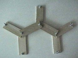
For the Brachts and Dembskis of the worlds, here is yet another physical analogy to make this crucial point clear. If the connections in the Genetic Algorithm are physically represented by wooden sticks of various lengths, and the nodes are physically represented by bolts that can be used to connect the sticks at their ends, then the “hypervolume” of possible solutions includes any and all arrangements of sticks, provided that the bolts used to connect the sticks have one of the five fixed positions, or any allowed “variable” position.
Here are two physical realizations of such networks - just two members of untold billions from the “hypervolume” of possible solutions. The first network here connects all fixed points, as required; it consists of 11 sticks joining the five fixed and four variable nodes (bolts), and has a (scaled) length of 2874 units. This is representative of the typical “organism on the street,” selected randomly from the vast hypervolume of solutions.

The second network also connects the fixed points, but with only seven sticks, with a total length of 1212 units. This “house-like” structure represents the formal Steiner Solution for the five-node system
When Bracht or Dembski say that Steiner Solutions are somehow implicitly imbedded in the fitness function, that’s like saying the specific design of a house is implicitly imbedded in the concepts of nails, lumber and economy. No, it’s not.
Other creationist/ID critics have written me to say that the desired answers were already present in the initial population, and that all my program was doing was removing “redundant” connections to reveal the best minimal networks. Sorry, but that doesn’t wash either. I tried to reduce the 2874-unit-long “monster” above by removing redundant connections. My first attempt got the length down to 1473 units (or 21% longer than the Steiner’s 1212).

I tried again, this time acheiving a length of 1368 units (or about 13% longer than the Steiner).

So, evolving solutions like the Steiner or the MacGyvers involves more than just knocking out some redundant segments of random networks. It really requires selection, reproduction, and mutation - just like real evolution.
Given a big pile of nails and lumber, it’s obvious that many different “houses” could be built by someone using the available hardware. The shape - the design - of the house is NOT spelled out in a loose assemblage of lumber and nails, not even if the person or “intelligence” who is to actually build the house understands that less lumber means lower cost.
CONCLUSION
The bottom line is that this simulation shows, once again, “how possibly” the basic processes of selection, mutation and sex, occurring over hundreds of generations, can result in some very striking innovations. That’s a reason that Genetic Algorithms are being increasingly used in industry.
In my algorithm, the Fitness Test is easy to apply: calculate the length of active segments. Shorter connected systems are more “fit.” In real life, the “fitness test” is likewise simple to apply: if an organism lives long enought to have offspring, it “passes”, otherwise it “fails.”
Despite the ID crowd’s claims to the contrary, Evolutionary Algorithms can produce produce striking novelty, without any pre-specifications of a “target.” While the Weasel and Hello World simulations are interesting in their own right, they are not intended as serious analyses of the real thing. Some simulations that study evolution seriously, like the Traveling Salesman Problem, are easily visualized. Others, like Avida, are more difficult to grasp on an intuitive level.
However, “Weasel” is not representave of all Genetic Algorithms, and there is simply no excuse for ID’s continuing “Bait and Switch” tactics as regard such algorithms.
And that’s why I’ve decided to release my Steiner MacGyvers on an unsuspecting world.
Will Dembski ever change his tune? Not likely, especially considering these comments from page 221 of No Free Lunch, regarding a genetic algorithm that was used to develop antennas given a fitness function that simply favored uniform gain:
A particularly striking example is the “crooked wire genetic antennas” of Edward Altshuler and Derek Linden. The problem these researchers solved with evolutionary (or genetic) algorithms was to find an antenna that radiates equally well in all directions over a hemisphere situated above a ground plane of infinite extent. Contrary to expectations, no wire with a neat symmetric geometric shape solves this problem. Instead, the best solutions to this problem look like zigzagging tangles. What’s more, evolutionary algorithms find their way through all the various zigzagging tangles–most of which don’t work–to one that actually does. This is remarkable. Even so, the fitness function that prescribes optimal antenna performance is well-defined and readily supplies the complex specified information that an optimal crooked wire genetic antenna seems to acquire for free.
Again, giving an engineer a pile of wire segments and instructions on “uniform gain” does not inherently specify the design of an optimal antenna, any more than the design of a house (or a Steiner network) is inherent in a pile of lumber and nails, even with instructions to “hold down lumber costs.”
As PT’s own Alan Gishlick, Nick Matzke, and Wesley R. Elsberry stated in Meyer’s Hopeless Monster,
While some genetic algorithm simulations for pedagogy do incorporate a “target sequence”, it is utterly false to say that all genetic algorithms do so. Meyer was in attendance at the NTSE in 1997 when one of us [WRE] brought up a genetic algorithm to solve the Traveling Salesman Problem, which was an example where no “target sequence” was available. Whole fields of evolutionary computation are completely overlooked by Meyer. Two citations relevant to Meyer’s claims are Chellapilla and Fogel (2001) and Stanley and Miikkulainen (2002). (That Meyer overlooks Chelapilla and Fogel 2001 is even more baffling given that Dembski 2002 discussed the work.) Bibliographies for the entirely neglected fields of artificial life and genetic programming are available at these sites:
http://users.ox.ac.uk/~econec/alife.html http://www.cs.bham.ac.uk/~wbl/biblio/gp-bibliography.html.
A bibliography of genetic algorithms and artificial neural networks is available here.
I’ve shown how one genetic algorithm, in the absence of a specific intended “target,” can produce multiple innovations for given network problems. But the ID/creationist crowd is still stuck on criticizing Dawkin’s “Weasel.”
Will Dembski/Berlinski et.al. ever take on, say, the Traveling Salesman Program, or the present work? Don’t hold your breath!
POSTSCRIPT: A BRIEF COMMENT ON DEMBSKI’S “NO FREE LUNCH” ARGUMENTS
Dembksi’s claims regarding the “No Free Lunch” theorem have been thoroughly fisked at the Thumb, here and here for example. His version of this theorem basically states that, when averaged over ALL POSSIBLE fitness functions, genetic algorithms do no better than chance. But that much is obvious. For example, if I had specified “longer is better” in my Genetic Algorithm - or not considered length at all - I would have not ended up with compact structures. (I know - I did the experiments!) Of course, thousands upon thousands of different “fitness tests” could be conceived. Averaging over all of these is irrelevant to the question at hand - what can be done with one simple fitness function? If you placed a large population of brown bears in a polar environment, and could wait long enough, you might see the bears evolve into white-furred animals like Polar Bears. But, if you averaged over all possible environments - polar, desert, mountaintop, marine, tundra, rainforest, etc. - you would not see the emergence of white-furred bears, not even after many millions of years. Evolution responds to the environment at hand, not fictional families of all possible environs. Dembski’s “No Free Lunch” claims are on the same “sound” mathematical foothold as his factoring of 59, or his understanding of normalization. (And Dembski’s been messing up so much lately, folks are piling on.)
POSTSCRIPT: SERIOUS USE OF ‘TARGETED’ SELECTION
Sometimes the concept of a “target” is used in real studies of the evolution of specific characters or traits, or combinations of those features. For example, D. Waxman and J.J. Welch (“Fisher’s Microscope and Haldane’s Ellipse”, American Naturalist, 166:447-457, 2005) describe the following type of fitness functions:
“In Fisher’s and Kimura’s analyses, it was assumed that all traits are under stabilizing selection of identical intensity. In particular, it was assumed that the fitness of a phenotype is a monotonically decreasing function of its Euclidean distance from the optimal phenotype. Geometrically, this corresponds to a “fitness landscape” that is spherically symmetric. “Surfaces” of constant fitness are hyperspheres (i.e., circles when n = 2, spheres when n = 3, …) that are centered on the optimal phenotype. If we choose to measure each trait in such a way that its optimal value is 0, then the optimal phenotype will lie at the coordinate origin, z = 0 = (0,0,…,0). Fitness is then a function of z = (z_1^2+z_2^2+…+z_n^2)^{1/2}.”
The point is not that “optimal phenotypes” or “targets” have no utility in any discussions of evolution. They certainly do, in the proper context. Rather, the point is that some computer analyses, and evolution itself, do not require any sneaking in of complex information beforehand.
A CHALLENGE TO ID ADVOCATES/CREATIONISTS
I have placed the complete listing of the Genetic Algorithm that generated the numerous MacGyvers and the Steiner solution, at the NMSR site.
If you contend that this algorithm works only by sneaking in the answer (the Steiner shape) into the fitness test, please identify the precise code snippet where this frontloading is being performed. The listing includes documentation on how the “Doggie” was geneticially engineered into certain experiments. For the main set of runs (no engineering), the “Doggie” codes were commented out (C or !).
FURTHER READING
Ian Musgrave’s Weasel Page: http://www.health.adelaide.edu.au/Pharm/Musgrave/essays/whale.htm
“Touched by nature: Putting evolution to work on the assembly line” by C. W. Petit (U.s. News & World Report) http://www.genetic-programming.com/published/usnwr072798.html
“36 Human-Competitive Results Produced by Genetic Programming” http://www.genetic-programming.com/humancompetitive.html
There are now 36 instances where genetic programming has produced a human-competitive result. … These human-competitive results include 15 instances where genetic programming has created an entity that either infringes or duplicates the functionality of a previously patented 20th-century invention, 6 instances where genetic programming has done the same with respect to a 21st-centry invention, and 2 instances where genetic programming has created a patentable new invention.
“Publications using Avida as a research platform” http://dllab.caltech.edu/pubs/